Context
This post is a continuation of an article, so it'd be ideal/nice if you read the first part of this post here: Tinker, smol-RL and QDoRA.
TLDR; (Part-1)
In Part 1, I showcase how reproducibility poses a practical problem in modern LLM work, not just a philosophical ideal. Even with greedy decoding and fixed seeds, determinism can break in subtle ways: GPU type, numerical precision, kernel choices, and non-deterministic log-probs in MoE models all conspire to make "run it again" less reliable than we like to admit. That led to a simple question: do we need a better abstraction layer so that the model ops complexity is hidden but the critical knobs for determinism are explicit and repeatable? Tinker reminded me of scikit-learn style API but for post-training models and the cookbook makes it easier to standardize the fragile pieces of post-training like reproducibility settings, dataset pre-processing, and stable training/inference pipelines. In Part 1, I talk about the Just-RL paper and how its a great starting point for testing Tinker's RLVR and RLHF setups on a small models before scaling data and model size.
Introduction
In this post I take the smallest possible bite out of the Part 1 plan: a zero-shot Qwen3-8B baseline on single-turn disruption classification, a pair of QDoRA SFT runs on the same task, and a before/after read that separates "the model can follow the JSON contract" from "the model can actually classify disruption." I then add a smaller SFT-vs-RL follow-up on Qwen3-4B-Instruct-2507 and gpt-oss-20b, using the repo's local src/sft and src/rl paths, to ask what the training signal is actually optimizing.
The simple version is: I first ask Qwen3-8B to do the task zero-shot under a strict JSON output contract, just to see what the base model can already do on its own. Then I run QDoRA SFT on the same prompt and task, first with 10k balanced examples and then with a 40k follow-up, so the change is easy to read without moving the goalposts. That gives a cleaner before-and-after story, not just on label accuracy, but also on per-class recall and calibration.
The later runs are less flattering but more useful. They show that an RL loop can keep the output contract mostly intact while still collapsing onto a single class, and that gpt-oss-20b can produce recoverable JSON while failing a raw strict evaluator because its completions include analysis-prefixed text before the JSON payload. That makes Part 2 less of a "bigger model + RL fixes it" story and more of a measurement story: the output parser, reward, and model family are all part of the experimental object.
Data
The setup also matters because these runs do not begin from a generic instruction-tuning dataset. The broader corpus behind the disruption experiments is a SciSciNet/OpenAlex-style paper collection with 1,972,797 records. At the metadata level, each record can carry fields like openalex_id, title, abstract, publication_year, cited_by_count, cd_index, novelty_score, conventionality_score, disruption_label, novelty_label, primary_field, and concepts. For the actual RL experiments, though, I used a fixed JSONL slice: data/sci_balanced_from2m_no_ovr.rl_balanced.jsonl. A quick polars pass gives the main shape of that file:
>>> import polars as pl
>>> df = pl.scan_ndjson("data/sci_balanced_from2m_no_ovr.rl_balanced.jsonl")
>>> df.collect_schema().names()
['openalex_id', 'title', 'abstract', 'publication_year', 'cited_by_count',
 'cd_index', 'novelty_score', 'conventionality_score', 'disruption_label',
 'novelty_label', 'primary_field', 'concepts']

>>> df.select(pl.len()).collect().item()
600000

>>> df.group_by("disruption_label")
... .agg(pl.len().alias("n"))
... .sort("disruption_label")
... .collect()
shape: (3, 2)
┌──────────────────┬────────┐
│ disruption_label ┆ n      │
│ ---              ┆ ---    │
│ str              ┆ u32    │
╞══════════════════╪════════╡
│ consolidating    ┆ 200000 │
│ disruptive       ┆ 200000 │
│ neutral          ┆ 200000 │
└──────────────────┴────────┘

>>> df.select(
...     pl.col("publication_year").min().alias("min_year"),
...     pl.col("publication_year").max().alias("max_year"),
...     pl.col("cited_by_count").median().alias("median_citations"),
...     pl.col("cited_by_count").quantile(0.9).alias("p90_citations"),
...     pl.col("cited_by_count").max().alias("max_citations"),
... ).collect()
shape: (1, 5)
┌──────────┬──────────┬──────────────────┬───────────────┬───────────────┐
│ min_year ┆ max_year ┆ median_citations ┆ p90_citations ┆ max_citations │
│ ---      ┆ ---      ┆ ---              ┆ ---           ┆ ---           │
│ i64      ┆ i64      ┆ f64              ┆ f64           ┆ i64           │
╞══════════╪══════════╪══════════════════╪═══════════════╪═══════════════╡
│ 1875     ┆ 2024     ┆ 12.0             ┆ 90.0          ┆ 21559         │
└──────────┴──────────┴──────────────────┴───────────────┴───────────────┘
That small block already says most of what matters for interpreting the later runs. The file is not a toy benchmark, but it is also not the full upstream corpus. It is a balanced 600k slice with 200k examples per disruption class, and each example carries enough structure to be more than plain text: title, abstract, year, citation count, field, and the citation-derived disruption label. In practice, though, the runtime loader narrows this further and only uses the six fields that matter for the disruption task: title, abstract, publication_year, cited_by_count, primary_field, and disruption_label.
The important point here is that these labels are not arbitrary buckets I made up for the RL loop. The disruption labels come from citation-network behavior, and the novelty/conventionality fields come from how unusual or familiar a paper's reference combinations look relative to the background literature. Even though the current RL sequence only uses disruption_label, the wider corpus already carries the fuller science-of-science structure.
For disruption, the intuition is: what do future papers do after they cite a focal paper? If later work cites the focal paper without also citing its references, the focal work looks more disruptive. If later work keeps citing the focal paper together with the papers it built on, the work looks more consolidating. Values near the middle behave more like neutral. The figure below is the cleanest visual explanation of that idea from Wu, Wang, and Evans, Large teams develop and small teams disrupt science and technology.
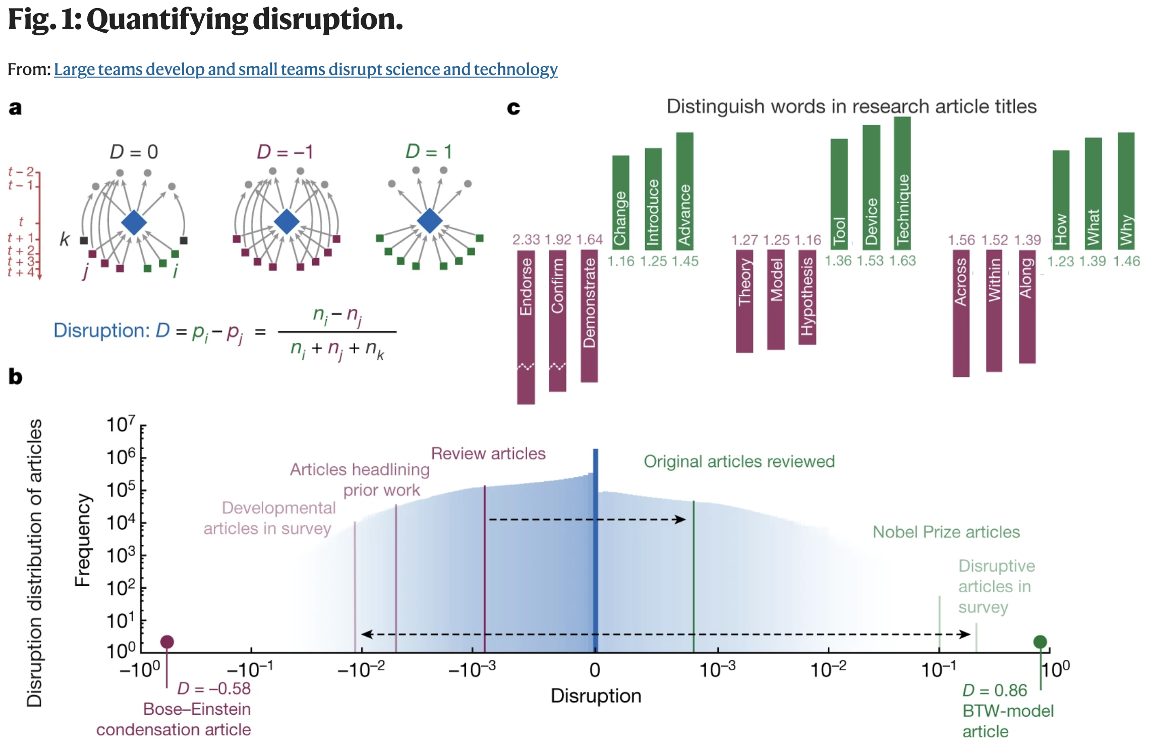
Fig. Reference view of disruption from Wu, Wang, and Evans, Large teams develop and small teams disrupt science and technology, Nature (2019).
That paper figure is the clean conceptual picture. For this post, though, the more useful question is: what does cd_index actually look like in the balanced JSONL that feeds the RL runs? The next plot recreates the panel b idea on the 600k slice used here. Two details matter. First, the slice is already balanced for training, so it should not be read as the natural frequency profile of the full 1.97M-paper source corpus. Second, the actual metadata thresholds in this dataset are much tighter than the older shorthand I used in Part 1: cd_index <= -0.001 is consolidating, -0.001 < cd_index < 0.001 is neutral, and cd_index >= 0.001 is disruptive. The tall spike at 0 is not a plotting bug; it is the empirical shape of the slice, where a large fraction of the neutral mass sits exactly at or extremely close to zero.
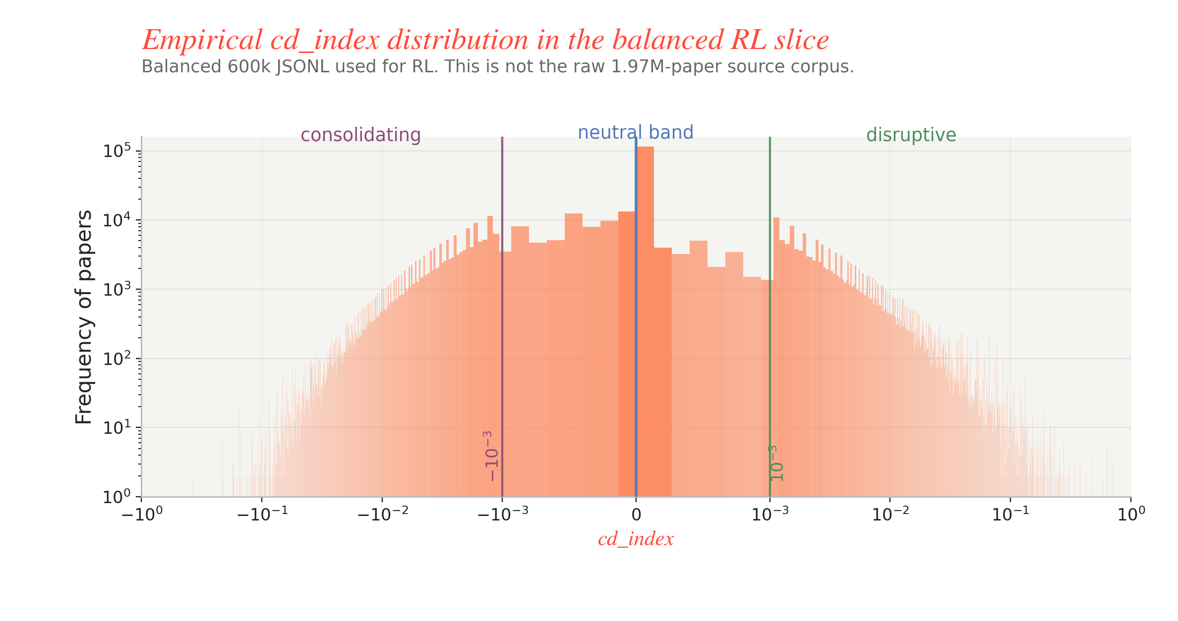
Fig. Dataset view of cd_index on the balanced 600k RL slice. The x-axis is shown on a signed log scale and the y-axis is paper frequency on a log scale; the shaded bands mark the dataset cutoffs for consolidating, neutral, and disruptive.
For novelty and conventionality, the logic is different. Here the question is not whether a paper overturns or develops prior citation pathways, but whether the combinations of prior work it cites are unusual or familiar. In the Uzzi et al. framing, the left tail corresponds to more novel combinations and the right side corresponds to more conventional combinations. That is why the corpus stores both novelty_score and conventionality_score: a paper can be mostly grounded in familiar prior work while still injecting a smaller amount of unusual combination. The figure below is from Uzzi et al., Atypical Combinations and Scientific Impact.
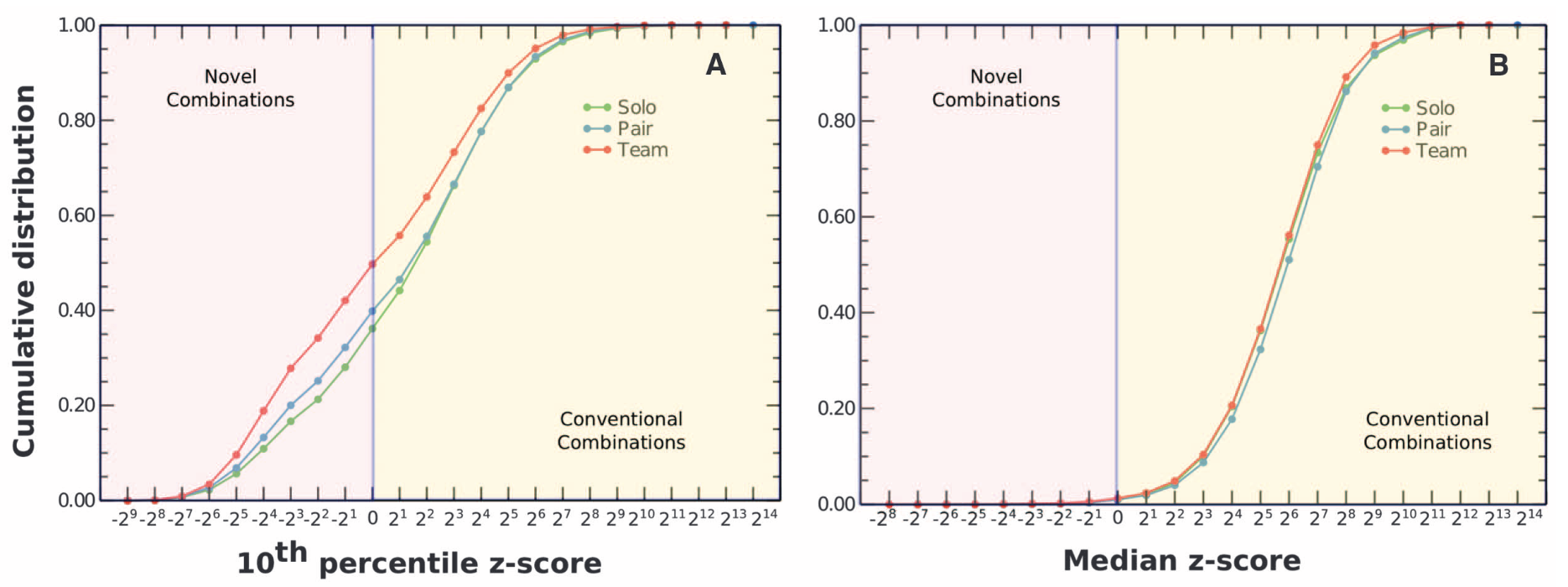
Fig. Reference view of novelty and conventionality from Uzzi et al., Atypical Combinations and Scientific Impact, Science (2013).
The broader provenance is still useful context. This balanced JSONL was carved out of a much larger SciSciNet/OpenAlex-style paper corpus with 1,972,797 records, where the raw disruption distribution is naturally skewed: about 247,090 papers are labeled disruptive, about 583,215 are consolidating, and about 1,142,492 are neutral. So the experiments here are not using the world as-is; they are using a balanced slice of a much more imbalanced scientific-impact distribution. That distinction ends up mattering quite a bit once the reward starts encouraging the model to exploit class asymmetries.
For this post, the zero-shot, SFT, and follow-up RL runs load this JSONL in the same spirit. A manifest-based split is attempted first, but its coverage against the RL-balanced JSONL is only about 30%, so the loader falls back to a deterministic 80/10/10 shuffle with seed = 2026 — giving 480000 train, 60000 val, and 60000 test rows. Held-out evaluations then subsample the first 2000 rows of val and the first 2000 rows of test, so every number in the next section is read against the same fixed 2000-row slices. The SFT runs use deterministic train subsets from the 480000-row train split; the RL runs use 5000 train examples and run for 250 GRPO steps.
For the SFT-vs-RL follow-up, I used the teacher-confidence variant of the same file, data/sci_balanced_from2m_no_ovr.rl_balanced.with_teacher_confidence.jsonl, because both the SFT target and the RL reward include the confidence field in addition to disruption_label. That means the model is not only being asked to classify disruption; it is also being asked to express calibrated confidence under a strict two-key JSON contract.
Experiment(s)
Zero-shot baseline
I first evaluated Qwen3-8B zero-shot through a local SGLang endpoint, using a strict JSON schema with two required keys, disruption_label and confidence. On the frozen 2000-row test slice, the model reaches label_match = 0.3525, macro_f1 = 0.3036, and parse_ok = 0.994. Most completions satisfy the output contract, but classification accuracy remains low, especially for disruptive papers.
| class | recall (test) | dominant confusion |
|---|---|---|
disruptive |
0.0358 |
→ neutral (398/698), consolidating (268) |
consolidating |
0.4749 |
→ neutral (281/617) |
neutral |
0.5650 |
→ consolidating (267/685) |
Table. Per-class recall and dominant confusion patterns for the zero-shot baseline on the frozen 2000-row test slice.
The model identifies only 25 of 698 disruptive papers. It assigns 398 to neutral and another 268 to consolidating. With errors this uneven across classes, an increase in aggregate accuracy alone would tell me little about whether a later training run improved disruptive-paper recall.
The model is also overconfident. The schema allows confidence values of low, medium, and high. Among the 1988 scored predictions, it emits high for 1893 and medium for 95, never using low. Mean predicted confidence is 0.786, mean accuracy is 0.355, and expected calibration error (ECE) is 0.431.
QDoRA SFT
I trained two supervised checkpoints with the same QDoRA configuration: DoRA at rank 64, alpha 128, and dropout 0.05 on the seven linear projections (q_proj, k_proj, v_proj, o_proj, gate_proj, up_proj, down_proj), over a 4-bit NF4 Qwen3-8B base with bf16 compute. Both runs use paged adamw_8bit with lr = 2e-5, a cosine schedule, warmup_ratio = 0.03, one epoch, per_device_train_batch_size = 1, and gradient_accumulation_steps = 4.
The first run uses a deterministic 10000-example subset of the 480000-row training split and finishes at step 2500. The second uses 40000 examples and finishes at step 10000. Evaluation uses greedy generation with max_new_tokens = 64 on the same frozen 2000-row validation and test slices. Increasing the training set therefore also increases the number of optimizer updates; this comparison measures the combined change.
The SFT targets include both disruption_label and confidence. The confidence target comes from |cd_index| magnitude, assigning high to papers far from the dataset's decision thresholds and low to ambiguous cases. This teaches the model a citation-derived proxy for confidence. Whether its reported confidence agrees with prediction accuracy still requires a separate calibration check.
Both checkpoints improve label accuracy and macro-F1 over the zero-shot baseline, while parse_ok remains at 0.994.
| run | final step | label_match |
macro_f1 |
parse_ok |
|---|---|---|---|---|
10k |
2500 |
0.573 |
0.577 |
0.994 |
40k |
10000 |
0.633 |
0.634 |
0.994 |
Table. Overall held-out test metrics for the two QDoRA SFT checkpoints.
| run | recall: disruptive |
recall: consolidating |
recall: neutral |
|---|---|---|---|
10k |
0.536 |
0.642 |
0.549 |
40k |
0.688 |
0.605 |
0.603 |
Table. Per-class recall on the same frozen 2000-row test slice for the two QDoRA SFT checkpoints.
The 10k checkpoint reaches similar label_match / macro_f1 values on validation (0.5635 / 0.5662) and test (0.573 / 0.5773). It also changes the distribution of errors. Among disruptive papers in the test slice, 248 are classified as consolidating and 69 as neutral. Disruptive recall rises to 0.536, although confusion between the two directional labels remains substantial.
At 40k, test label_match increases from 0.573 to 0.633, and macro_f1 from 0.577 to 0.634. Disruptive recall shows the largest gain (0.536 → 0.688), followed by neutral recall (0.549 → 0.603). Consolidating recall falls from 0.642 to 0.605, with 174 consolidating papers classified as disruptive, up from 147. The larger run identifies more disruptive papers at the cost of more false disruptive predictions among consolidating papers.
Both SFT checkpoints use the low confidence category and have lower ECE than the zero-shot baseline. For the 10k run, mean predicted confidence is 0.359, mean accuracy is 0.576, and ECE is 0.253. Its 1452 low-confidence predictions reach 0.522 accuracy; its 520 high-confidence predictions reach 0.733.
For the 40k run, mean predicted confidence rises to 0.385 and mean accuracy to 0.637, while ECE increases to 0.285. The 573 high-confidence predictions reach 0.742 accuracy, and the 1334 low-confidence predictions reach 0.593. On this test slice, 40k produces the better classifier and 10k has the lower calibration error. Both now report mean confidence below mean accuracy, so the reduction in zero-shot overconfidence comes with underconfidence on average.
SFT-vs-RL follow-up
I next compared SFT and RL on Qwen3-4B-Instruct-2507 and gpt-oss-20b to examine how each training signal affects classification and output validity. The task requires the model to return valid JSON and distinguish disruptive, consolidating, and neutral papers. I evaluate these requirements separately because a parseable answer can still assign the wrong label.
The follow-up consists of four runs:
| experiment | model | training signal | what it tests |
|---|---|---|---|
exp1_qwen4b_sft | Qwen/Qwen3-4B-Instruct-2507 | supervised JSON targets | classification and JSON validity after SFT on the smaller Qwen model |
exp2_qwen4b_rl | Qwen/Qwen3-4B-Instruct-2507 | GRPO reward | classification and JSON validity after RL on the same model family |
exp3_gptoss20b_sft | openai/gpt-oss-20b | supervised JSON targets | strict output validity and JSON recovery after SFT |
exp4_gptoss20b_rl | openai/gpt-oss-20b | GRPO reward | strict output validity and JSON recovery after RL |
The Qwen SFT run produced a validation checkpoint at step 2500, but its test evaluation is unavailable. I report the validation result here, with the test comparison still incomplete. The other three runs completed with final held-out evaluations.
| run | validation result | observed behavior |
|---|---|---|
exp1_qwen4b_sft |
label_match=0.5165macro_f1=0.5152parse_ok=0.993 |
All three classes have nonzero validation recall; test performance remains unmeasured. |
exp2_qwen4b_rl |
label_match=0.3405macro_f1=0.1700parse_ok=0.991 |
Almost all predictions are neutral, with valid JSON on most rows. |
exp3_gptoss20b_sft |
parse_ok=0.0clean_parse_ok=0.3345label_match=0.0 |
The strict scorer rejects every completion because analysis text precedes the JSON. |
exp4_gptoss20b_rl |
parse_ok=0.0clean_parse_ok=0.9995label_match=0.0 |
The clean parser recovers JSON on almost every row; the strict scorer rejects all rows. |
Table. SFT and RL results on the fixed 2000-row validation slice. For gpt-oss-20b, clean_parse_ok measures JSON recovery from completions that the strict parser rejects because analysis text precedes the JSON object.
Supervised training helped Qwen distinguish the citation-derived classes. The clearest evidence comes from the earlier Qwen3-8B runs: disruptive recall increased from 3.6% zero-shot to 68.8% after SFT on 40k examples. The smaller Qwen SFT checkpoint also identified examples from all three classes on validation, although its test evaluation is still missing.
The Qwen3-4B RL run returned valid JSON on about 99% of test examples, but predicted neutral for almost everything. Its roughly 34% accuracy came entirely from neutral papers. It correctly identified none of the disruptive or consolidating papers. For a task intended to distinguish these citation patterns, this policy offers little beyond assigning the same label to every paper.
GPT-OSS is harder to assess because the evaluator rejects its output before checking the labels. After RL, the clean parser recovered JSON from 99.95% of test completions. Analysis text preceding the JSON still caused every completion to fail strict scoring. The resulting zero score tells us that the output failed the required format; the accuracy of the recovered labels remains unmeasured.
Before extending these RL runs, I would score the recovered GPT-OSS labels and test whether changes to the Qwen reward improve disruptive and consolidating recall without sacrificing neutral recall. That would let me assess whether RL helps distinguish the citation patterns this task is meant to measure.
References
1. https://arxiv.org/pdf/2402.03300
2. https://arxiv.org/pdf/2205.01833
3. https://arxiv.org/pdf/2402.09353
4. https://www.science.org/doi/10.1126/science.1240474
5. https://www.nature.com/articles/s41586-019-0941-9
Cite
@misc{akhil2026notesdrnote2,
  author       = {Akella, Akhil Pandey},
  title        = {Tinker, smol-RL and QDoRA (Part 2)},
  year         = {2026},
  month        = {February},
  url          = {https://akhilpandey95.github.io/notes/tinker_part2/},
  note         = {Accessed: }
}